Rank-Based Clustering for Improved Pipeline Performance

The DuckDB team wrote a great post on why you might worry about the write order in tables prepared for analytical purposes: Faster Dashboards with Multi-Column Approximate Sorting. It's a great introduction to space-filling curves and why they're relevant for optimizing queries that could target multiple columns - well worth a read. The gist is that the multiple columns used for some downstream purpose (e.g. querying or joins) form a multi-dimensional space, but the row order - imperative for skipping row groups - is inherently one-dimensional. The task for optimizing for multi-column queries becomes one of effectively reducing this multi-dimensional space to a one-dimensional order.

Getting this right is especially important for multi-step data transformation pipelines, where the same table might be used for multiple purposes downstream.

The key insight of this article is that space-filling the potential values in the dataset is sub-optimal for an uneven distribution of values. By first ranking the values from each column, and interleaving those ranks, much better performance can be achieved. This is especially valuable where it's fine for a row's key to change as the table does, such as when the whole table is rewritten. Here I present a variety of alternative methods for comparison on the TPC-DS dataset.

Why order matters for query performance

In a Parquet file, rows are grouped into chunks called row groups (DuckDB writes 122,880 rows per group by default), and within each group every column is stored and compressed separately. Alongside the data, the file's footer records statistics for each column in each row group, including its smallest and largest value. If you ask for WHERE price BETWEEN 400 AND 430, DuckDB reads the footer first, and any row group whose price range is, say, 2 to 380 can't possibly contain a match. DuckDB skips it without decompressing a byte. These per-group ranges are often called zone maps.

If rows are ordered randomly (the worst case), every row group contains a similar distribution of values. Every footer's min/max values are nearly identical, spanning the full set of values, so no query can avoid reading everything.

If only one column is required downstream, then ordering by that column does a fantastic job (theoretical best) at splitting the row groups - for a unique column, any target value could only exist in exactly one row group. For multiple columns though, there is a trade off - ordering first by the first 'most important' column might mean the second column is barely ordered at all (depending on the first's cardinality). Typical lexicographic ordering like this can help very little if the columns are not selected carefully.

Row group skipping under multiple orders

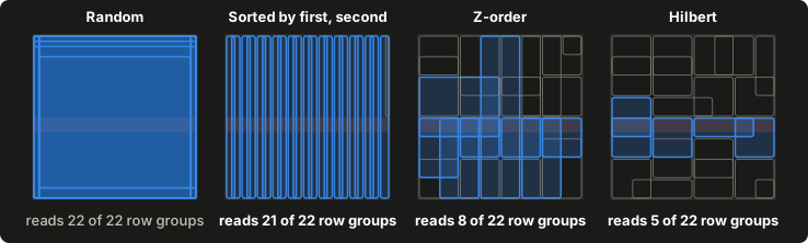
Shaded band is the filter, blue boxes are candidate row groups, unshaded boxes are skipped row groups.

The figure above shows the problem on a toy table: every cell of a 32 by 32 grid, written in four different orders and split into row groups of 48 rows. Each box is one row group's min/max range, and the shaded band is a filter on the second column. In random order every box spans the whole grid, so all 22 row groups are read. Sorting by the first column and then the second gives tall, thin stripes - ideal for a filter on the first column, but a filter on the second still reads 21 of the 22.

Space-filling curves for dimension reduction

Space-filling curves are a mathematical construction that threads a one-dimensional path (curve) through a higher-dimensional space. They are self-similar at various scales, and as their fidelity increases, they enable these higher-dimensional spaces to be mapped entirely by the path. This is very useful in multiple fields, due to these mappings approximately preserving proximity in the higher-dimensional space when condensed down to the single dimension path.

The Hilbert curve is a particularly beautiful variant, where each step is adjacent to the previous - a property that also makes it more effective for the purpose of dimension reduction. The Morton 'Z-order' however is used more commonly, as its construction is very straightforward: the first bit of the first column is taken, then the first of the second, and so on, then the second bit of the first column, until some bit depth is reached or the data is exhausted - a process called 'bit-interleaving'. This has the neat effect of drawing a series of 'Z' shapes, themselves ordered into 'Z' shapes, snaking their way through the multi-dimensional space.

Curve visualization

Morton and Hilbert curves in two dimensions.

Both visit every cell only once, but the Z-order makes long jumps at the edge of each quadrant - row groups that cover either end of these extremes have very poor separation. The Hilbert curve, comparatively, only ever steps to a neighbouring cell. The question for which to use comes down to whether the extra complexity of evaluating the Hilbert curve is justified by performance improvements.

Rank-space vs value-space

Consider two columns of 4-bit values. Each value may be one of 16 possibilities, and bit-interleaving the pair gives $2^{4+4} = 256$ possible ordering values. This might be a perfectly good structure, if the true values in the data span the entire range of possibilities. In practice, values are rarely spread evenly across this potential value-space, and are instead clustered around some set of common values. If, say, only the first and last quarters of the possible values are used in each column (0 to 3, 12 to 15), the order curve will assume values 3 and 12 are distant, despite being adjacent in the true data.

Consider instead taking any two columns, ordering each, and breaking each into 16 equal-sized chunks, where each chunk is assigned a 4-bit value. This creates a rank-space, which necessarily better approximates the distribution of real data. The labels for these groups may then be interleaved to create the order key.

This is particularly valuable where there is real skew to the data. Here's ss_net_paid from TPC-DS, the amount paid per sale line, split into 16 buckets both ways:

Rows per bucket for ss_net_paid, 16 buckets

Scaled between its min and max, 58% of rows land in the first bucket and the top half of the range is nearly empty. The curve can only order rows by their buckets, so for most of the table this column contributes almost nothing to the order.

Beyond ordering, I've found these generated keys quite useful. Taking the first bit alone approximately halves the data, two bits quarters and so on. Values that have proximal keys are proximal in the higher-dimensional space, for the columns that were used to generate the key, allowing for some very rudimentary clustering analysis. In many cases where I would otherwise be producing a unique single column composed of multiple keys (a proxy key for composite keys), where one might otherwise use a hash, I've found using these keys to be more space-efficient and meaningful, with the bonus of providing a natural row order and partitioning axis.

Throughout this article, I'll call the value-space ordering simply "Morton" and "Hilbert", and the rank-space variants "rank-Morton" and "rank-Hilbert", respectively. In my own use, I've been calling it a 'mash', as a replacement for a hash - though given the ranks change with each evaluation, it's not appropriate for every situation. Given its ability to approximate the higher-dimensional distribution - or its manifold - a viable backronym might be "Manifold-Approximate Sorting Hierarchy". But, let's stick to the rank-* naming here!

This isn't an entirely new idea. Delta Lake's OPTIMIZE ... ZORDER BY passes each column through a function called range_partition_id, which its source describes as "an approximate rank() function", before interleaving the bits, and its Liquid Clustering uses the same ranks with a Hilbert curve.

Testing setup

I generated TPC-DS at scale factor 100 with DuckDB's tpcds extension and took the store_sales fact table: 288 million rows, 14.4 GB of Parquet. I then wrote it in each of these orders, with 122,880-row row groups (DuckDB default):

Order	Description
Random	sorted by a hash of the primary key
Sorted	a plain ORDER BY over the clustering columns
Morton, Hilbert	the curve over each column scaled between its min and max
Rank-Morton, rank-Hilbert	the curve over each column's quantile rank

I clustered on two sets of columns. The first pairs ss_sold_date_sk with the skewed ss_net_paid. The second is three surrogate keys (ss_sold_date_sk, ss_item_sk and ss_customer_sk), which are spread fairly evenly. Each layout then ran the same seeded set of reads: ranges on each column selecting 0.1%, 1% and 10% of rows, boxes over all of the clustering columns, and a few joins in the style of TPC-DS. This article reports only the 1% results, but you can see the other results in the benchmark directory. The metric to pay attention to is the 'share of rows read' - the proportion of the table's rows that could not be skipped. This is then independent of hardware.

Query time is the median of five warm runs on a 10-core laptop with 32 GB of memory, using DuckDB 1.5.

Theory

Measured by rank, every clustered column is spread evenly between the minimum and maximum. Assuming independence, for $k$ clustered columns, this forms a $k$-dimensional unit cube, with rows spread evenly through it. Correlation between columns allows better performance - for the TPC-DS dataset used in these tests, the columns are near independent.

Each of the $N$ row groups holds $1/N$ of the rows, so the box spanned by its min/max values has a volume of at least $1/N$. A range query selecting a fraction $s$ of one column is a slab of width $s$ through the cube, and a row group has to be read whenever its box overlaps the slab. For a row group whose box spans a width $w$ along that column, that happens with probability $s + w$, so the expected share of rows read is $s$ plus the average width of the row groups along that column.

If every clustered column matters equally, the quantity to minimise is that average width across all $k$ columns. For boxes of a fixed volume, it's smallest when every side is equal - a cube with a side of $N^{-1/k}$. So, averaged across the clustered columns, no layout can read less than:

$$s + N^{-1/k}$$

A layout can beat this for one column by favouring it - lexicographic ordering reads close to $s$ for its first column, but at the expense of the others. For the SF100 tests, with $N = 2{,}344$ row groups, the bound for a 1% range is 3.1% with two clustered columns and 8.5% with three.

Lowest possible share of rows read for a 1% range

The bound $s + N^{-1/k}$ for $k$ clustered columns. The dashed line is $s = 1\%$, the matching rows themselves.

Results

Ranking helps with skew

Share of rows read, clustered on (ss_sold_date_sk, ss_net_paid)

TPC-DS SF100, 288M rows, 2,344 row groups. Lower is better.

In this test, a range query for 1% of ss_sold_date_sk values, and separately a range query for 1% of ss_net_paid, was executed for clusters based on (ss_sold_date_sk, ss_net_paid).

As expected, the random order does not manage to skip any row group at all, and 100% of the data is read for both the ss_sold_date_sk and ss_net_paid ranges.

The ss_sold_date_sk column has around 1,800 distinct values across 288M rows, resulting in around one per row group. That doesn't give much room for ss_net_paid to do much to the order beyond that. Ordered lexicographically, the result is optimal performance on the ss_sold_date_sk range at 1%, but poor performance on ss_net_paid at 82% of rows read.

The Morton and Hilbert (value-space) orders do a much better job at supporting queries on ss_net_paid, cutting it down to 12-16% and sacrificing little to the performance against ss_sold_date_sk. This would be much better though, if not for the significant skew in ss_net_paid. The rank-space methods bring both queries to within the 3-5% range - close to the theoretical best of 3.1%.

Fewer rows read translates fairly directly into faster reads. With a warm cache, the 1% ss_net_paid range goes from about 200 ms in random order to 19 ms in rank-Hilbert order:

Query time for a 1% range on ss_net_paid

TPC-DS SF100, median of 5 warm runs, for a count and a sum over the matching rows.

These are warm-cache timings on a local SSD, so they measure the decoding and filtering that DuckDB avoids. When reading from object storage, where every skipped row group is a request that never has to be made, I'd expect the gap to be wider.

Hilbert beats Morton on performance

Share of rows read for a 1% range, clustered on (ss_sold_date_sk, ss_item_sk, ss_customer_sk)

TPC-DS SF100. Lower is better.

Using instead three non-skewed columns, the value-space and rank-space methods are around the same. However, Hilbert consistently beats Morton for the lowest-importance ss_customer_sk column, giving 9-10% across the board, against a theoretical best of 8.5%. Hilbert is worthwhile where there's a need for all included columns to be approximately equally-weighted.

Calculation and writing costs

Rank-Hilbert is the clear winner when it comes to performance, but evaluating the curve is complex. Its use over Morton is only justified if it's not too expensive to create, though in many cases this operation can be done rarely to mitigate the cost (e.g. during compaction of a large dataset into cold storage).

Time to write the clustered table

TPC-DS SF100, clustered on (ss_sold_date_sk, ss_net_paid), 7 bits per column. One run each.

This shows the results of one run - note that between-run variation was around 20%, so much of the performance difference is hidden behind noise. The ranks need not be exact, so the ranking part of the process used approximate quantiles.

Writing the table without sorting took around 30 seconds. The lexicographic sort approximates the minimum that could be expected by any sorted write, taking around 160 seconds - anything beyond this is likely the evaluation time. Morton added around 20s, while rank-Morton was another 20s beyond that. The ranking itself appears to cost around 20s - though closer to 12s when measured directly below.

Interestingly, rank-Hilbert took around the same time as rank-Morton, indicating that the difference in evaluation costs is well below the noise.

As each row's key depends only on its own values, DuckDB is able to stream the calculation rather than requiring the entire table to be held in memory. The memory costs are therefore surprisingly light. Evaluating the approx_quantile pass and key calculation cost directly, to disentangle from sort costs:

Key	Time	Peak memory
Morton	3.6 s	130 MB
Hilbert	7.1 s	150 MB
Rank-Morton	16 s	220 MB
Rank-Hilbert	20 s	260 MB

From a memory perspective there is minimal difference. Compared to Morton, the Rank-Hilbert method adds no more than 20% to total write time.

Sorting within files

The Delta Lake implementation doesn't sort rows within a file by default. It range-partitions rows into files by the curve key, so each file covers a slice of the curve, and leaves the rows inside each file unordered. That makes sense for Delta, which records each file's min and max in its transaction log and skips whole files without opening them - on object storage, that saves a request per file. I tried the same, partitioning into files of 256 MB and 1 GB:

Share of rows read when sorting inside files, or only between them

TPC-DS SF100, rank-Hilbert key on (ss_sold_date_sk, ss_net_paid). Lower is better.

It saved 25 to 40% of the write time, but read 4 to 8 times more rows with 256 MB files, and more again with 1 GB files. DuckDB prunes at the row group, inside the file, so for DuckDB most of the benefit comes from the order within each file. When DuckDB is the reader, it's worth sorting the whole thing.

Trying it in plain DuckDB

None of this needs anything special. Here's the same approach in plain DuckDB SQL, ranking with approx_quantile and walking the ranks with the lindel community extension's hilbert_encode, which the DuckDB post also uses:

INSTALL lindel FROM community;
LOAD lindel;

COPY (
    WITH bounds AS (
        SELECT
            approx_quantile(ss_sold_date_sk, [i / 64 FOR i IN range(1, 64)]::FLOAT[]) AS d,
            approx_quantile(ss_net_paid,     [i / 64 FOR i IN range(1, 64)]::FLOAT[]) AS p
        FROM store_sales
    )
    SELECT s.*
    FROM store_sales s, bounds
    ORDER BY hilbert_encode([
        len(list_filter(d, b -> b < s.ss_sold_date_sk)),
        len(list_filter(p, b -> b < s.ss_net_paid))
    ]::UTINYINT[2])
) TO 'store_sales_clustered.parquet';

The list_filter count is each row's bucket: the number of boundaries its value sits above. 64 buckets per column makes 4,096 cells on the grid, which suits a table of a few thousand row groups. It's worth aiming for roughly one cell per row group, since finer cells can't help a min/max check. On TPC-DS at scale factor 10 this clustered 29 million rows in about 6 seconds, and a 1% range on ss_net_paid then read 23 of 235 row groups. NULLs land in bucket 0 here, which is fine for most tables.

In Duckstring

As of v0.6.1 of Duckstring, cluster_by uses the rank-Hilbert order described here. The columns to cluster on are declared when a table is written:

pond.merge_table("sales", rows, pk="ticket_id", cluster_by=["sold_date", "net_paid"])

For merge tables this applies only during compaction, which occurs any time a table's warm, freshness-tagged data exceeds the existing cold, compacted data (after reaching a minimum size). That keeps recent data recency-ordered (which tends to be most useful in incremental pipelines), and older data rank-Hilbert-ordered. For overwritten tables (using pond.write_table()), it's applied at every write.

Duckstring picks the number of buckets from the table's size, so that each cell is just under one row group. It keeps a separate bucket for NULLs, uses exact quantiles for tables under ten million rows (so small tables come out identical every time) and approximate ones above that. The guide has additional details.

Summary

• In Parquet, the single row order matters enormously for query performance, especially against multiple columns.
• The Hilbert curve outperforms Morton Z-order slightly, and lexicographic sort dramatically.
• Ranking each column before mapping helps address skew and unevenness.
• Write and evaluation times are mild against the minimum time to order.
• In DuckDB, sorting within files is generally worthwhile.